Pairs Trading in the Cryptocurrency Market
We apply the fundamental Spread model, ARIMA model, XGBoost, and LSTM to implement pairs trading for cryptocurrency. We analyze 10 pairs with the largest market capitalization of the crypto market, resulting in locking on utilizing the pair: ADA-USD, and XRP-USD as the pair’s cointegration results suit our strategy the most. The critical strategy that we have implemented is the mean reverting strategy, in order to present high-robustness trading, we combined with the ARIMA model, XGBoost, and LSTM respectively to deal with the time-series prediction. In the end, we conducted a backtest and displayed the return for each strategy, all of them delivering great profitability.
Introduction
Pairs Trading is a typical and popular market-neutral trading strategy, it could potentially help investors make profits regardless of whether the market is bullish or bearish and was first utilized by certain intelligent analysts at Morgan Stanley in the 1980s. There exist several different editions of pairs trading in the market, in this project, the authors focus on the statistical arbitrage trading strategy, which pays attention to the ideas of cointegration and assumes self-error correction in the equity market.
The fundamental idea to earn gains in the capital market is to buy the underpriced stock and sell the overpriced stock, but evaluating a certain stock’s intrinsic value is difficult. In recent days, people have started to apply Machine Learning methods to the prediction of stock prices. However, due to the high noise and target drift in the trading data, the Machine Learning method will usually treat the stock prediction as a classification problem. When considering the classification problem, industries will usually adopt the method of Deep Learning, but this is an end-to-end process, which means that the input is the original data, the output is directly the final target, and the intermediate process is unknowable. In this regard, Deep Learning has been criticized as a Black Box system that performs well but does not present a credible reason, in other words, it lacks explanation.
In contrast, pairs trading aims to solve the difficulty of predicting a certain stock’s price by using the idea of relative pricing based on the arbitrage pricing theory (APT) in finance. It is a common way to construct a portfolio by a certain smooth linear combination which is also called a cointegration function, after which, the spread will be a mean-reverting stationary process. Under this condition, our target is to produce a positive return as valuations converge based on the spread when there exists mispricing.
The pivot for a pairs trading strategy is to select a proper pair of financial instruments. During periods of heightened volatility, assets usually have a tendency to become more correlated, even if they are in different sectors, the cryptocurrency presents representatively high volatility, so the authors decide to investigate this market. However, only the correlation between the two prices may not be good enough for a good pair. In reality, a good pair should have the same characteristics and risk exposure, in this project, the authors choose the biggest 10 market capitalization currencies, utilizing the cointegration test to pitch on the pair of ADA and XPR because of its smallest corresponding p-values.
Since the spread has been a mean-reverting and stationary process as discussed previously, the authors not only take spread price into consideration but also tried to apply several different models and methods to help generate trading signals, such as ARIMA (Autoregressive integrated moving average), XGBoost (Extreme Gradient Boosting), and LSTM (Long short-term memory networks).
Implementation of Pure Mean-reverting Strategy
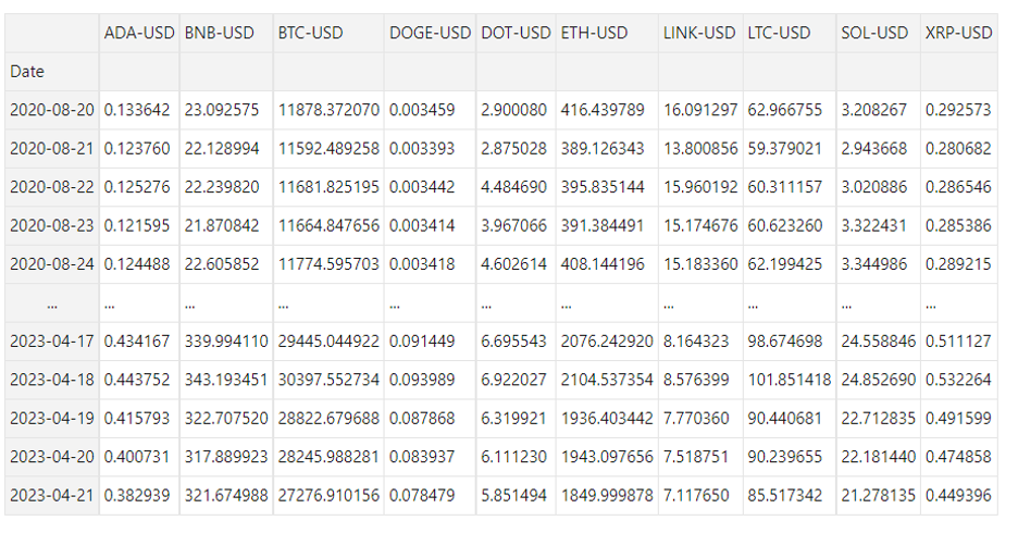
We downloaded the top ten cryptocurrencies’ daily trading data especially the closed price with the largest market capitalization: BTC, ETH, BNB, ADA, DOGE, XRP, SOL, DOT, LTC, and LINK, all to the USD pairs by Yahoo Finance API. The time frame is set from 2020-08-20 to 2023-04-21, as the most recent bull market round started in the year 2020.
import yfinance as yf
from IPython.display import clear_output
import pandas as pd

# top 10 cryptos
cryptos = ['BTC-USD', 'ETH-USD', 'BNB-USD', 'ADA-USD', 'DOGE-USD', 'XRP-USD',
           'SOL-USD', 'DOT-USD', 'LTC-USD', 'LINK-USD']

#start and end dates for the data, change if necessary
start_date = '2020-01-01'
end_date = '2023-04-22'

# data for each crypto
crypto_data = yf.download(cryptos, start=start_date, end=end_date)

# Close price for each crypto
prices = crypto_data['Close'].dropna()
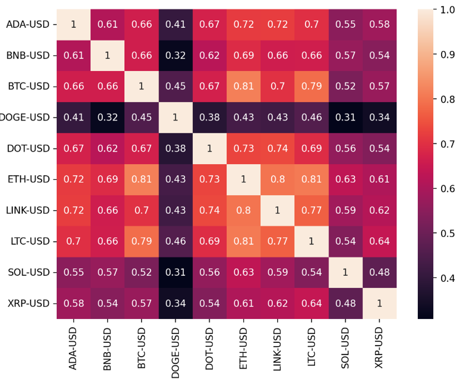
We took the log returns of each currency pair, then calculated the correlation between each pair, which allowed us to assess their linear relationship. The correlation of the crypto market is generally higher than that of the stock market. For example, during periods of extreme market volatility, such as the crypto market crash in 2018, many cryptocurrencies experienced significant price declines in a similar pattern.
To make the result visually intuitive, we represented the correlation matrix using a heatmap, where darker colors indicate lower correlations and brighter colors indicate higher correlations.
# dalily log return
return_corr = np.log(prices/prices.shift(1)).dropna().corr()
plt.figure(figsize=(8, 6), dpi=200)
sn.heatmap(return_corr, annot = True)
Pairs Selections (Augmented Engle-Granger two-step cointegration test):
Furthermore, in order to make the selection of a more informative pair, it is necessary to compute the cointegration for each pair by utilizing the closed prices of the cryptocurrencies directly, which accounts for the long-term relationship between them. Since the keys to pairs trading involve identifying whether the pair has a stable long-term relationship, we adopted the j to compute the p-value on each of the pairs, and as the same for correlation, we also computed a heat map.
While there are many dark areas in the heat map that indicate small p-values, we eventually selected a pair with the lowest number; they are ‘ADA-USD’, and ‘XRP-USD’ with a p-value of 0.0002.
Pure Mean Reverting:
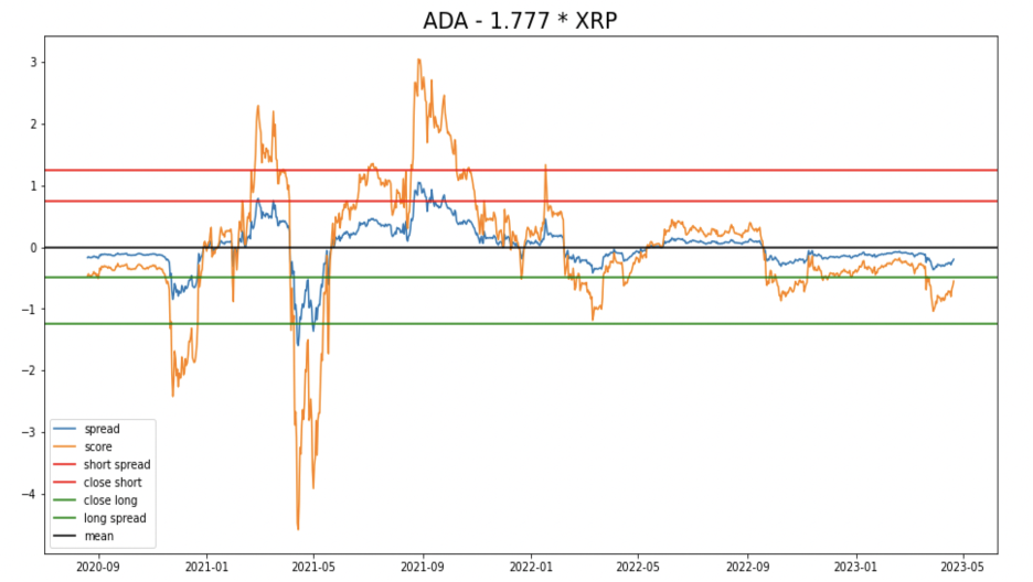
After selecting a cointegrated pair of ADA and XRP, we construct a spread by using the linear combination \(w_t=p_1t-γp_2t\) of these two assets. The general idea behind a pairs-trading strategy is to trade on the oscillations about the equilibrium value of the spread because the spread is mean reverting. Therefore, if the spread is getting bigger, we can conclude that the magnitude of mispricing is larger, and so is the potential profitability.
Under this framework, we sell the overpriced crypto, and buy the underpriced crypto, assuming that the mispricing will correct itself in the future. In this project, we use the following standardized score as the fundamental trading strategy signal, the score is calculated by the formula: (current spread value - mean of spread value)/(standard deviation of spread value).
Since positive values indicate the value is above the mean, and vice versa. If the score > 1.25, we short the spread (short ADA, long XRP), when the score value falls back to 0.75, we buy to recover the position, same logic for the other hand, if the score < -1.25, we choose to enter a short position and close it when scoring < -0.5.
The trading principle is as follows: When there exists a trading signal, first place half of the wealth into the long position of the pair, while at the same time opening a short position in the other pair based on the calculated hedge ratio. The available wealth is determined by adding the cash balance and the value of the portfolio.
This is a diagram of visualization of our spread and score, however, it is just a template because it runs a linear regression on the whole two years’ data.
Linear regression on the entire dataset may not give a good fit between the two, so we implement the following strategy. We run linear regression and find the proper hedge ratio every 30 days, utilizing it to trade for the following 7 days. The algorithm is shown as below: For the day i from 1 to end-30:
- Find spread
- If the hedge ratio is negative, i =i+1 (pass this trading cycle), else:
- If the spread is nonstationary (implement the Augmented Dickey–Fuller (ADF) test), i = i+1 else:
- make a trading decision according to the score for the i+31th day
- i = i+1
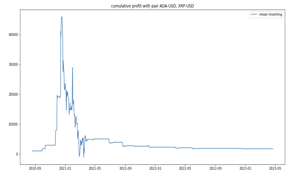
This is the cumulative profit diagram of the pure mean-reverting strategy, in our trading time horizon, the wealth increases from $1000 to $1740, but the max-drawdown is extremely high.
Modified mean-reverting strategy
TBC