Portfolio optimization with stochastic dominance constraints
A study of the problem of constructing a portfolio of finitely many assets
We study the problem of constructing a portfolio of finitely many assets whose return rates are described by a discrete joint distribution. In particular, we study the portfolio optimization via stochastic dominance constraints in the second order.
Introduction
The Portfolio Problem
Let \(R_1, R_2,..., R_n\) be random return rates of assets \(1,2,...,n\). We assume that \(\mathbb{E}[|R_j|] \le \infty\) for all \(j=1,...,n.\)
Our aim is to allocate our capital in these assets in order to obtain the desirable total return rate on the investment. Denoting by \(x_1, x_2,..., x_n\) be the weights of the initial capital invested in the corresponding assets \(R_1, R_2,..., R_n\). Therefore, the total return rate is:
\[\begin{equation} R(x) = R_1 x_1 + R_2 x_2 + \dots + R_n x_n \end{equation}\]We consider the set of possible asset allocations as follows:
\[\begin{equation} X = \{x \in \mathbb{R}^n: x_1 +x_2 + \dots + x_n = 1, \ x_j \geq 0, j=1,2, \dots, n\}. \end{equation}\]Notice that all \(x_j\) are nonnegative, i.e., we do not consider allocations where we have short positions in the portfolio. Clearly, it is a convex polyhedron.
The main difficulty in formulating a meaningful portfolio optimization porblem is the definition of the preference structure among feasible portfolios. If we only consider
\[\begin{equation} \mu(x) = \mathbb{E}[R(x)], \end{equation}\]then resulting optimization problem has a trivial solution: invest everything in assets that have the maximum expected return rate. For these reasons the portfolio optimization resorts usually to two approaches. The first approach is to associate the portfolio $x$ with some dispersion measure \(\rho(R(x))\) which represents the variability of the return rate $R(x)$. The function
\[\rho(R(x))\]is the variance of the return rate,
\[\rho(R(x)) = \mathbb{V} ar[R(x)].\]The mean-risk portfolio optimization problem is formulated as follows:
\[\begin{equation*} \underset{x \in X}{\text{max}} \quad \mathbb{E}[R(x)] - \lambda \mathbb{V} ar[R(x)] \end{equation*}\]The second approach is to select a certain utility function \(u: \mathbb{R} \rightarrow \mathbb{R}\) and to formulate the optimization problem:
\[\begin{equation*} \underset{x \in X}{\text{max}} \quad \mathbb{E}[u(R(x))] \end{equation*}\]It is usually required that the function \(u(*)\) is concave and nondecreasing, thus reflecting preferences of a risk-averse decision maker. The challenge in utility approaches is to select appropriate utility function to represents our preferences because of the fact that it is almost impossible to elicit the utility function of a decision maker explicitly.
In this blog, we study an alternative approach, by introducing a comparison to a benchmark return rate into the optimization problem. This approach has a fundamental advantage over both mean-risk models and utility function models. All data for our model are readily available. In mean-risk models the choice of the risk measure has an arbitrary character \(\lambda\), and it is difficult to argue for one measure against another. Optimization of expected utility requires the form of the utility function to be specified. The alternative approach, departing from the benchmark outcome, generates implied utility function of the decision maker.
Stochastic Dominance
Direct Forms
In the stochastic dominance approach, random return rates are compared by a pointwise comparison of some performance functions constructed from their distribution functions. Consider a random variable \(X \in \mathcal{L}^1(\Omega, \mathcal{F}, P)\) and the first performance function is defined as its distribution function
\[F(X; \eta) = P[X \leq \eta] \quad for \quad \eta \in \mathbb{R}\]A random return \(X\) is said to stochastically dominate another random return \(Y\) in the first order, denoted \(X \succeq_{(1)} Y\) if
\[F(X; \eta) \leq F(Y; \eta)\]The second performance function \(F_2(X;*)\) is defined as
\[F_2(X;\eta) = \int_{-\infty}^{\eta} F(X;\alpha) d \alpha \quad for \quad \eta \in \mathbb{R}\]A random return \(X\) is said to stochastically dominate another random return \(Y\) in the second order, denoted \(X \succeq_{(2)} Y\) if
\[F_2(X; \eta) \leq F_2(Y; \eta).\]There are many properties of the second performance function, one of the most important related to our model is the following.
The theory of stochastic orders plays a fundamental role in economics. It has an equivalent characterization in terms of the expected utility theory. A random variable $R$ dominates the random variable \(Y\) if \(\mathbb{E}[u(R)] \geq \mathbb{E}[u(Y)]\) for all functions \(u(*)\) from certain set of functions.
- Stochastic dominance of first order is defined by the set of nondecreasing function: A random variable \(R\) dominates the random variable \(Y\) of first order if \(\mathbb{E}[u(R)] \geq \mathbb{E}[u(Y)]\) for all nondecreasing functions \(u(*)\) defined on \(\mathbb{R}\).
- Stochastic dominance of second order is defined by the set of nondecreasing and concave function: A random variable \(R\) dominates the random variable \(Y\) of second order if \(\mathbb{E}[u(R)] \geq \mathbb{E}[u(Y)]\) for all nondecreasing and concave functions \(u(*)\) defined on \(\mathbb{R}\).
Thus, no risk-averse decision maker will prefer a portfolio with return rate $Y$ over a portfolio with return rate $R$ if $R$ dominate $Y$ of second order.
The following further illustrate the relations between second order dominance constrains and the utility function models. Let us consider the set \(\mathcal{U}\) of concave nondecreasing function \(u: \mathbb{R} \rightarrow \mathbb{R}\) satisfying the following linear growth condition:
\[\begin{equation*} \lim_{t \to -\infty} u(t)/t < \infty \end{equation*}\]Suppose that \(X \succeq_{(2)} Y\), we have
\[\mathbb{E}[(\eta -X)_{+}] \geq \mathbb{E}[(\eta -Y)_{+}] \quad {\mbox{for all }} \eta \in \mathbb{R},\]It follows that that for all functions of the form
\[u_N(x) = c_N - \sum_{i=1}^N \alpha_i (\eta_x -x)_+ ,\]where \(\alpha_i \geq 0, i =1,...,N,\) We have
\[\begin{equation} \mathbb{E}[u_N(X)] \geq \mathbb{E}[u_N(Y)] \ \ \ \ \ \ (1) \end{equation}\]Let \(u \in \mathcal{U}.\) We construct sequence of functions of the above form \({u_N}\) to approach \(u\). For an integer M, we have the discretization points
\[\begin{equation*} \eta_i = i/M, \quad -M^2 \leq i \leq M^2 \end{equation*}\]and we define \(c_M = u(M)\), and
\[\begin{equation*} \alpha_i =\left\{ \begin{array}{ccc} \frac{u(\eta_i) - u(\eta_{i-1})}{\eta_i - \eta_{i-1}} & \text{if} & i = M^2 \\ \frac{u(\eta_i) - u(\eta_{i-1})}{\eta_i - \eta_{i-1}} -\frac{u(\eta_{i+1}) - u(\eta*{i})}{\eta_{i+1} - \eta_{i}} & \text{if} & i = M^2-1, M^2-2,..., -M^2 +1 \\ u(\eta_i) - u(\eta_i -1) - \frac{u(\eta_{i+1}) - u(\eta_{i})}{\eta_{i+1} - \eta\_{i}} & \text{if} & i = -M^2 \end{array}% \right. \end{equation*}\]By construction, the function
\[u_M(x) = c_M - \sum_{i=-M^2}^{M^2} \alpha_i (\eta_x -x)_+ ,\]is a piecewise linear approxiamtion of u with nodes \((\eta_iu(\eta_i)), i = -M^2,..., M^2.\) By dominant convergence theorem, we have
\[\lim_{M \to \infty} \mathbb{E}[u_M(X)] = \mathbb{E}[u(X)], \quad for \ all \ X \in \mathcal{L}^1(\Omega, \mathcal{F}, P).\]Therefore, by taking limits on both sides of (1), we have
\[\begin{equation*} \mathbb{E}[u(X)] \geq \mathbb{E}[u(Y)] \end{equation*}\]On the other hand, if the above is true, then it is true for particular functions \(u(x) = -(\eta -x)_+\),
The Dominance-Constrained Portfolio Problem
The starting point for our model is the assumption that a benchmark random return Y having a finite expected value is available. It may have the form of \(Y=R(z)\), for some benchmark portfolio \(z\). Indeed, we will consider this kind of portfolio in our numerical illustration. It may also be an index or our current portfolio. Therefore, we study the following extension of the mean-risk optimization problem:
\[\begin{equation*} \begin{aligned} & \underset{x}{\text{max}} & & \mathbb{E}[R(x)] - \lambda \mathbb{V} ar[R(x)] \\ & \text{subject to} & & R(x) \succeq_{(2)} Y, \\ & & & X \in C \end{aligned} \end{equation*}\]To simplify the derivations, we focus on the simplest formulation of the dominance-constrained problem:
\[\begin{equation*} \begin{aligned} & \underset{x}{\text{max}} & & \mathbb{E}[R(x)]\\ & \text{subject to} & & R(x) \succeq_{(2)} Y, \\ & & & X \in C \end{aligned} \end{equation*}\]By Proposition (1), we further have the following version of the problem
\[\begin{equation} \label{expected} \begin{aligned} & \underset{x}{\text{max}} & & \mathbb{E}[R(x)] \\ & \text{subject to} & & \mathbb{E}[(\eta -X)_{+}] \geq \mathbb{E}[(\eta -Y)_{+}] \quad {\mbox{for all }} \eta \in \mathbb{R}, \\ & & & X \in C \end{aligned} \end{equation}\]Now we introduce a decision vector \(S\), to represent the shortfall and split the constrain in the above. The optimization becomes:
\[\begin{equation} \label{split} \begin{aligned} & \underset{x}{\text{max}} & & f(x) \\ & \text{subject to} & & X(\omega) + S(\eta,\omega) \geq \eta \\ & & &\mathbb{E}[S(\eta,\omega)] \leq \mathbb{E}[(\eta -Y)_{+}] \quad {\mbox{for all }} \eta \in \mathbb{R}, \\ &&& S(\eta,\omega) \geq 0 \\ & & & X \in C \end{aligned} \end{equation} \ \ \ \ \ \ \ \ \text{(*)}\]Let us assume now \(Y\) has a discrete distribution with realizations \(y_i\) attained with probabilities \(\pi_i, \ i=1,2,...m\). We also assume assume that the return rates have a discrete joint distribution with realizations \(r_{jt}, t=1,...,T, j=1,...,n\) attained with probabilities \(\pi_t, t=1,2,...T.\) Then the formulation of the problem () simplifies even further. Introducing variables \(s_{it}\) representing the shortfall of \(R(x)\) below \(y_i\) in realization \(t,i=1,2,...m,t=1,...,T,\) we can formulate the problem () as follows:
\[\begin{equation}\label{discrete} \begin{aligned} & \underset{x}{\text{max}} \sum_{t=1}^{T}pt \sum_{j=1}^n x_j r_{jt} \\ & \text{subject to} \\ & \sum_{j=1}^n x_j r_{jt} \geq y_i, \quad i =1,...,m \quad t = 1,...,T \\ & \sum_{t=1}^T p_t s_{it} \leq \sum_{k=1}^m \pi_k (y_i - y_k)_+ , \quad i =1,...,m \\ & s\_{it} \geq 0 \\ & x \in C \end{aligned} \end{equation}\]Indeed, for every feasible point of problem (*), by setting
\[s_{it} = max \left(0, y_i - \sum_{j=1}^n x_j r_{jt} \right), \quad i =1,...,m, \quad t = 1,...,T\]we obtain a feasible pair \((x,s)\) for problem (*). Conversely, for any feasible pair \((x,s)\) for problem above, the first two inequalities imply that \(s_{it} \geq max \left(0, y_i - \sum_{j=1}^n x_j r_{jt} \right), \quad i =1,...,m, \quad t = 1,...,T\) Taking the expected value of both sides and using the second inequalities, we obtain \(F_2(R(x); y_i) \leq F_2(Y; y_i).\) Therefore, the problem (1) is equivalent to problem above.
Numerical Illustration
In this section, we investigate whether the traditional 60/40 portfolio, i.e., 60% stocks with 40% bonds, is the optimal combination among others. The two assets are widely used:S\&P 500 and U.S. long term government bonds. We use the returns in successive quarters as equally probable realizations from 04/2009- 01/2020.
In other words, the reference random return Y has realizations:
\[y_t = \frac{6}{10} r_{1t} + \frac{4}{10} r_{2t} \quad t =1,2,...,m\]where m=43, and \(r_{1t}, r_{2t}\) denote the return of S&P 500 and U.S. long term government bonds respectively. The probabilities of these realizations are \(\frac{1}{43}\). The expected return of the reference portfolio is equal to 2.37%.
Our object is to maximize the expected return of the portfolio, under the condition that its return dominates the reference return Y in the second order.
The optimization problem above can be formulated as the following linear programming problem:
\[% \begin{equation}\label{discrete} \begin{aligned} & \underset{x}{\text{max}} \sum_{t=1}^{43} \sum_{j=1}^2 p_t x_j r_{jt} \\ & \text{subject to} \\ & \sum_{j=1}^2 x_j r_{jt} \geq y_i, \quad i =1,...,43 \quad t = 1,...,43 \\ & \sum_{t=1}^{43} p_t s_{it} \leq \sum_{k=1}^{43} \frac{1}{43} (y_i - y_t)_+ , \quad i =1,...,43 \\ & s\_{it} \geq 0 \\ & x_1 + x_2 =1, \quad x_1 \geq 0, \quad x_2 \geq 0 \end{aligned} % \end{equation}\]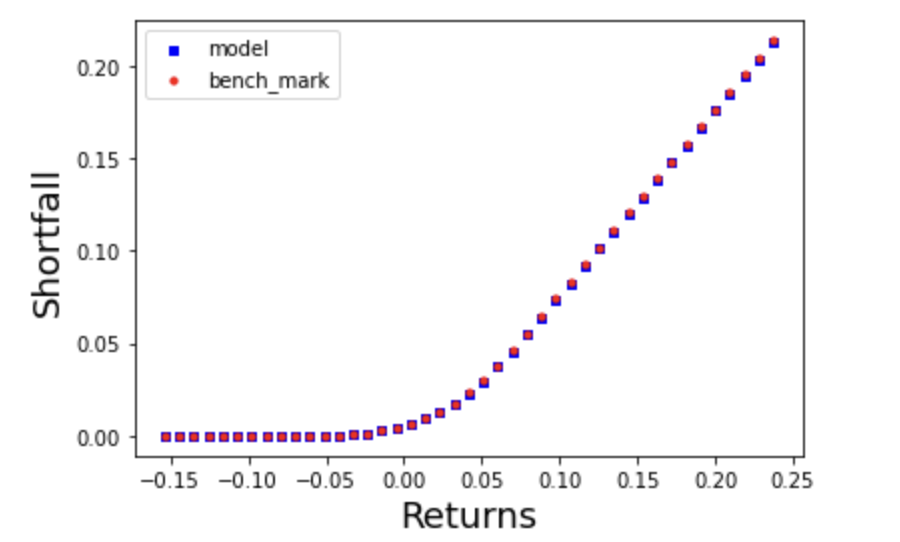
The optimal portfolio is
\[\left[0.64132052, 0.35867948\right]\]and it has expected return 2.46%. It is slight above the reference return and is much below the maximum expected return of 3.2% if we invest 100% on S&P 500. As we can also see, the portfolio is only slightly different from the benchmark \([0.6,0.4]\).
The expected shortfall \(F(X,*)\) appearing in the dominance constrains are illustrated in the Figure above. As we can see, the two portfolio shortfall functions largely overlap.
Reference
-
Dentcheva, Darinka., & Ruszczyński, Andrzej., Optimization with Stochastic Dominance Constraints. SIAM Journal on Optimization 14, 548–566.
-
Dentcheva, Darinka., & Ruszczyński, Andrzej., Portfolio optimization with stochastic dominance constraints. Journal of Banking & Finance Volume 30, Issue 2, February 2006, Pages 433-451.
-
Dentcheva, Darinka., & Ruszczyński, Andrzej., Risk-Averse Portfolio Optimization via Stochastic Dominance Constraints. Handbook of Quantitative Finance and Risk Management.
-
Ogryczak, Wlodzimierz., & Ruszczyński, Andrzej., From stochastic dominance to mean-risk models: Semideviations as risk measures. European Journal of Operational Research 116 (1999).
Check out PDF version below